Data Wrangling with dplyr
Tidyverse
There are a few key ideas to be aware of about how the tidyverse works in general before we dive into dplyr
Tidyverse
There are a few key ideas to be aware of about how the tidyverse works in general before we dive into dplyr
- Packages are designed to be like grammars for their task. You can string these grammatical elements together to form more complex statements, just like with language.
Tidyverse
There are a few key ideas to be aware of about how the tidyverse works in general before we dive into dplyr
Packages are designed to be like grammars for their task. You can string these grammatical elements together to form more complex statements, just like with language.
The first argument of (basically) every function is
data. This is very handy, especially when it comes to piping.
Tidyverse
There are a few key ideas to be aware of about how the tidyverse works in general before we dive into dplyr
Packages are designed to be like grammars for their task. You can string these grammatical elements together to form more complex statements, just like with language.
The first argument of (basically) every function is
data. This is very handy, especially when it comes to piping.Variable names are usually not quoted (read more here)
Palmer penguins
library(palmerpenguins)glimpse(penguins)## Rows: 344## Columns: 8## $ species <fct> Adelie, Adelie, Adelie, Adelie, Adelie, Adelie, Adelie, Adelie, Adelie, Adel…## $ island <fct> Torgersen, Torgersen, Torgersen, Torgersen, Torgersen, Torgersen, Torgersen,…## $ bill_length_mm <dbl> 39.1, 39.5, 40.3, NA, 36.7, 39.3, 38.9, 39.2, 34.1, 42.0, 37.8, 37.8, 41.1, …## $ bill_depth_mm <dbl> 18.7, 17.4, 18.0, NA, 19.3, 20.6, 17.8, 19.6, 18.1, 20.2, 17.1, 17.3, 17.6, …## $ flipper_length_mm <int> 181, 186, 195, NA, 193, 190, 181, 195, 193, 190, 186, 180, 182, 191, 198, 18…## $ body_mass_g <int> 3750, 3800, 3250, NA, 3450, 3650, 3625, 4675, 3475, 4250, 3300, 3700, 3200, …## $ sex <fct> male, female, female, NA, female, male, female, male, NA, NA, NA, NA, female…## $ year <int> 2007, 2007, 2007, 2007, 2007, 2007, 2007, 2007, 2007, 2007, 2007, 2007, 2007…dplyr
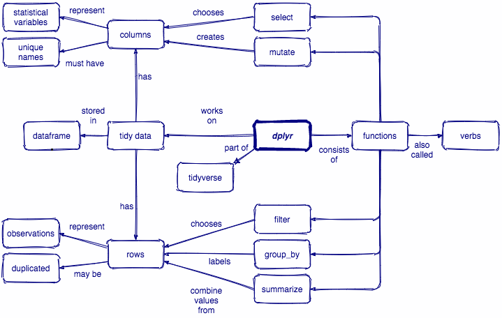
dplyr is a grammar of data manipulation, providing a consistent set of core verbs that help you solve the most common data manipulation challenges
dplyr
dplyr is a grammar of data manipulation, providing a consistent set of core verbs that help you solve the most common data manipulation challenges
Manipulating observations
filter()picks cases based on their values.arrange()changes the ordering of the rows.
dplyr
dplyr is a grammar of data manipulation, providing a consistent set of core verbs that help you solve the most common data manipulation challenges
Manipulating observations
filter()picks cases based on their values.arrange()changes the ordering of the rows.
Manipulating variables
select()picks variables based on their names.mutate()adds new variables that are functions of existing variables
Summarizing data
summarise()reduces multiple values down to a single summary.
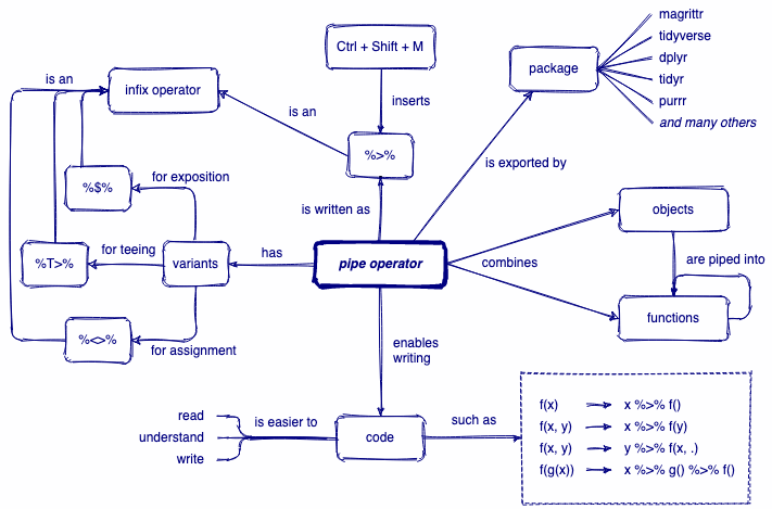
A review of pipes
x %>% f(y) is equivalent to f(x, y)
A review of pipes
x %>% f(y) is equivalent to f(x, y)
R Code
penguins %>% filter(species == "Gentoo") %>% select(bill_length_mm, bill_depth_mm) %>% arrange(desc(bill_length_mm))A review of pipes
x %>% f(y) is equivalent to f(x, y)
R Code
penguins %>% filter(species == "Gentoo") %>% select(bill_length_mm, bill_depth_mm) %>% arrange(desc(bill_length_mm))Translated into English
start with penguins data *AND THEN* filter to include only observations from Gentoo penguins *AND THEN* select only the columns `bill_length_mm` and `bill_depth_mm` *AND THEN* arrange observations by descending order of `bill_length_mm`A review of pipes
x %>% f(y) is equivalent to f(x, y)
R Code
penguins %>% filter(species == "Gentoo") %>% select(bill_length_mm, bill_depth_mm) %>% arrange(desc(bill_length_mm))Translated into English
start with penguins data *AND THEN* filter to include only observations from Gentoo penguins *AND THEN* select only the columns `bill_length_mm` and `bill_depth_mm` *AND THEN* arrange observations by descending order of `bill_length_mm`Read more on piping: https://magrittr.tidyverse.org/reference/pipe.html
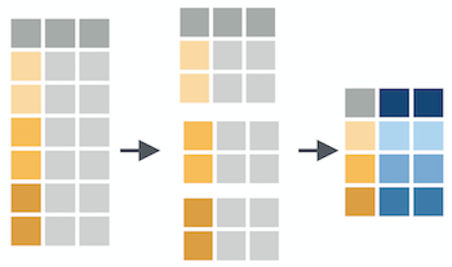
Manipulating observations
(rows)
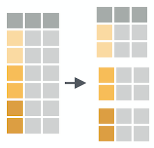
filter()
Subset observations (rows) with filter()

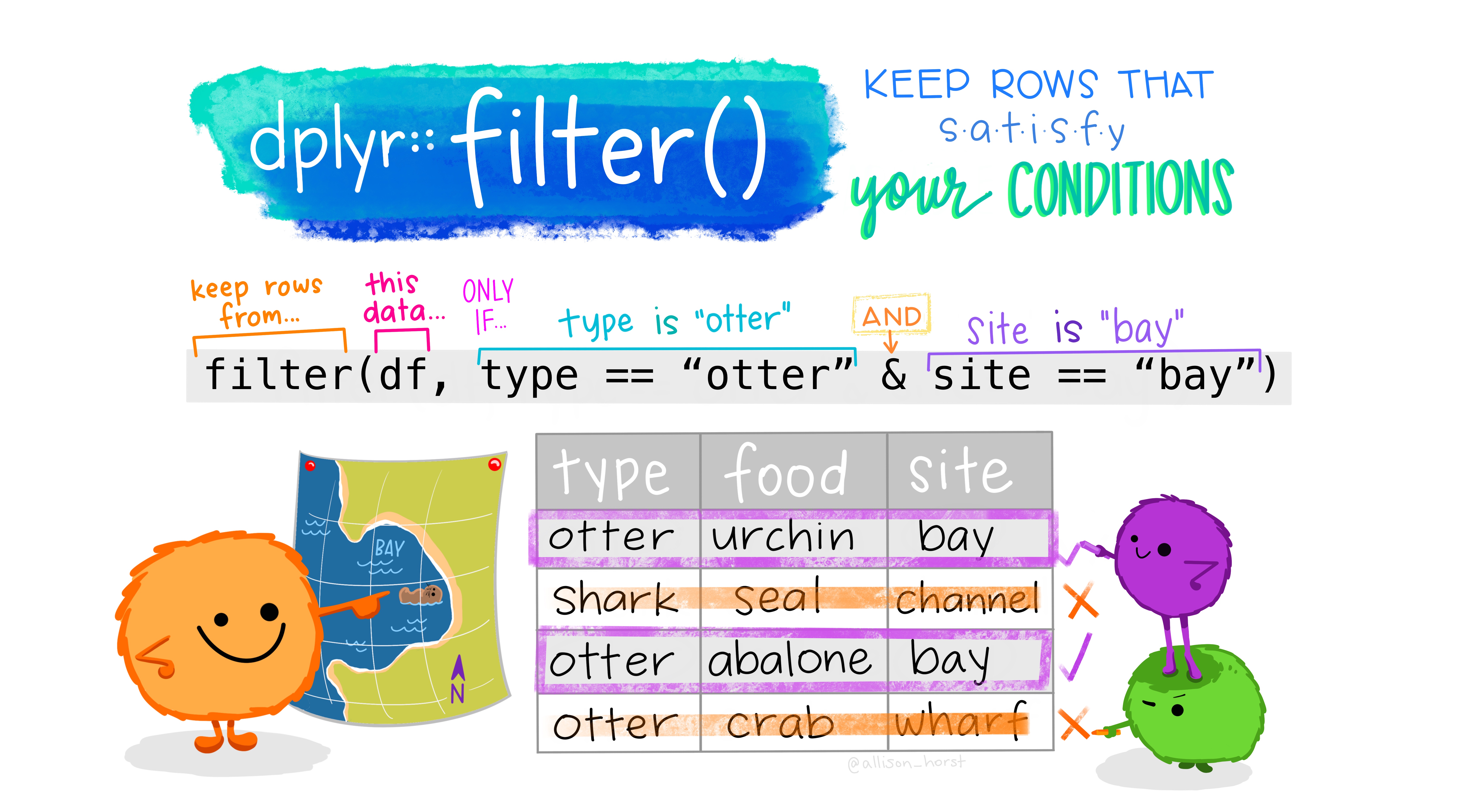
filter()
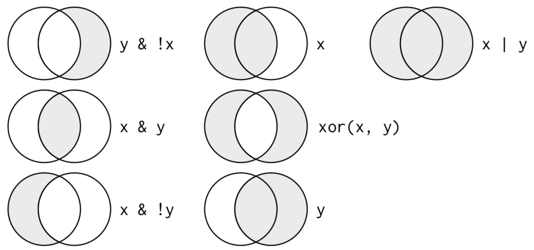
Comparisons
| Operator | Description | Usage |
|---|---|---|
| < | less than | x < y |
| <= | less than or equal to | x <= y |
| > | greater than | x > y |
| >= | greater than or equal to | x >= y |
| == | exactly equal to | x == y |
| != | not equal to | x != y |
| %in% | group membership | x %in% y |
| is.na | is missing | is.na(x) |
| !is.na | is not missing | !is.na(x) |
Source: Alison Hill
filter()
filter(.data, ...)
.data = a data frame or tibble
. . . = Expressions that return a logical value, and are defined in terms of the variables in .data.
If multiple expressions are included, they are combined with the & operator. Only rows for which all conditions evaluate to TRUE are kept.
penguins %>% filter(species == "Gentoo" & bill_length_mm > 55)## # A tibble: 3 x 8## species island bill_length_mm bill_depth_mm flipper_length_mm body_mass_g sex year## <fct> <fct> <dbl> <dbl> <int> <int> <fct> <int>## 1 Gentoo Biscoe 59.6 17 230 6050 male 2007## 2 Gentoo Biscoe 55.9 17 228 5600 male 2009## 3 Gentoo Biscoe 55.1 16 230 5850 male 2009penguins %>% filter(species %in% c("Adelie", "Gentoo"), island %in% c("Dream", "Torgersen"))## # A tibble: 108 x 8## species island bill_length_mm bill_depth_mm flipper_length_mm body_mass_g sex year## <fct> <fct> <dbl> <dbl> <int> <int> <fct> <int>## 1 Adelie Torgersen 39.1 18.7 181 3750 male 2007## 2 Adelie Torgersen 39.5 17.4 186 3800 female 2007## 3 Adelie Torgersen 40.3 18 195 3250 female 2007## 4 Adelie Torgersen NA NA NA NA <NA> 2007## 5 Adelie Torgersen 36.7 19.3 193 3450 female 2007## 6 Adelie Torgersen 39.3 20.6 190 3650 male 2007## 7 Adelie Torgersen 38.9 17.8 181 3625 female 2007## 8 Adelie Torgersen 39.2 19.6 195 4675 male 2007## 9 Adelie Torgersen 34.1 18.1 193 3475 <NA> 2007## 10 Adelie Torgersen 42 20.2 190 4250 <NA> 2007## # … with 98 more rows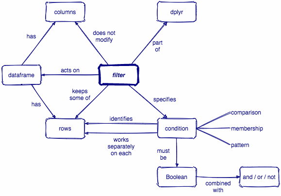
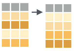
arrange()
Arrange rows by column values with arrange()
arrange()
arrange(.data, ...)
.data = a data frame or tibble
. . . = Variables to sort by. Use desc() to sort a variable in descending order.
penguins %>% filter(species == "Gentoo" & bill_length_mm > 55) %>% arrange(body_mass_g)## # A tibble: 3 x 8## species island bill_length_mm bill_depth_mm flipper_length_mm body_mass_g sex year## <fct> <fct> <dbl> <dbl> <int> <int> <fct> <int>## 1 Gentoo Biscoe 55.9 17 228 5600 male 2009## 2 Gentoo Biscoe 55.1 16 230 5850 male 2009## 3 Gentoo Biscoe 59.6 17 230 6050 male 2007penguins %>% filter(species == "Gentoo" & bill_length_mm > 55) %>% arrange(desc(body_mass_g))## # A tibble: 3 x 8## species island bill_length_mm bill_depth_mm flipper_length_mm body_mass_g sex year## <fct> <fct> <dbl> <dbl> <int> <int> <fct> <int>## 1 Gentoo Biscoe 59.6 17 230 6050 male 2007## 2 Gentoo Biscoe 55.1 16 230 5850 male 2009## 3 Gentoo Biscoe 55.9 17 228 5600 male 2009Your turn 1
05:00
Import the file
pragmatic_scales_data.csv(use best practices of a project-oriented workflow). Save it to an object calledps_data. This time we'll save it as atibble(which I've done for you).Filter rows for cases in the "No Label"
conditionand arrange the resulting observations by descending order ofage.Select observations from the “No Label” condition for kids 3 years old or younger.
Select observations for kids between the ages of 3 and 4. Save the result to a new object called
ps_filtered. (For an extra challenge, look up the documentation forbetween()and use this function instead of comparison operators).
Solution
# Q1.ps_data <- rio::import(here::here("data", "pragmatic_scales_data.csv")) %>% as_tibble()# Q2.ps_data %>% filter(condition == "No Label") %>% arrange(desc(age))## # A tibble: 288 x 5## subid item correct age condition## <chr> <chr> <int> <dbl> <chr> ## 1 SCH23 faces 0 4.82 No Label ## 2 SCH23 houses 0 4.82 No Label ## 3 SCH23 pasta 0 4.82 No Label ## 4 SCH23 beds 0 4.82 No Label ## 5 SCH1 faces 0 4.82 No Label ## 6 SCH1 houses 0 4.82 No Label ## 7 SCH1 pasta 0 4.82 No Label ## 8 SCH1 beds 0 4.82 No Label ## 9 SCH19 faces 0 4.79 No Label ## 10 SCH19 houses 0 4.79 No Label ## # … with 278 more rows# Q3.ps_data %>% filter(condition == "No Label" & age >= 3)## # A tibble: 192 x 5## subid item correct age condition## <chr> <chr> <int> <dbl> <chr> ## 1 SCH35 faces 0 3.02 No Label ## 2 SCH35 houses 0 3.02 No Label ## 3 SCH35 pasta 0 3.02 No Label ## 4 SCH35 beds 0 3.02 No Label ## 5 MSCH40 faces 0 3.02 No Label ## 6 MSCH40 houses 1 3.02 No Label ## 7 MSCH40 pasta 0 3.02 No Label ## 8 MSCH40 beds 1 3.02 No Label ## 9 SCH34 faces 0 3.06 No Label ## 10 SCH34 houses 0 3.06 No Label ## # … with 182 more rows# Q4. ps_filtered <- ps_data %>% filter(age >= 3 & age <= 4)ps_filtered## # A tibble: 204 x 5## subid item correct age condition## <chr> <chr> <int> <dbl> <chr> ## 1 T10 faces 0 3 Label ## 2 T10 houses 1 3 Label ## 3 T10 pasta 1 3 Label ## 4 T10 beds 1 3 Label ## 5 T3 faces 1 3.09 Label ## 6 T3 houses 1 3.09 Label ## 7 T3 pasta 1 3.09 Label ## 8 T3 beds 1 3.09 Label ## 9 T6 faces 1 3.1 Label ## 10 T6 houses 1 3.1 Label ## # … with 194 more rows# Q4.ps_filtered <- ps_data %>% filter(between(age, 3, 4))ps_filtered## # A tibble: 204 x 5## subid item correct age condition## <chr> <chr> <int> <dbl> <chr> ## 1 T10 faces 0 3 Label ## 2 T10 houses 1 3 Label ## 3 T10 pasta 1 3 Label ## 4 T10 beds 1 3 Label ## 5 T3 faces 1 3.09 Label ## 6 T3 houses 1 3.09 Label ## 7 T3 pasta 1 3.09 Label ## 8 T3 beds 1 3.09 Label ## 9 T6 faces 1 3.1 Label ## 10 T6 houses 1 3.1 Label ## # … with 194 more rowsManipulating variables
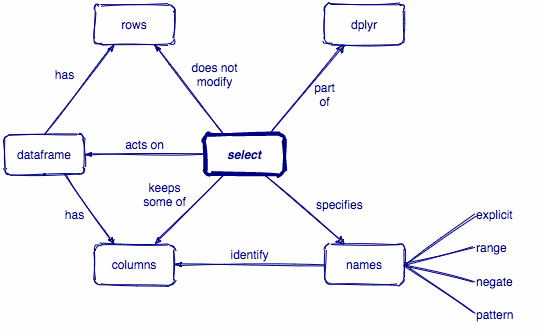
(columns)
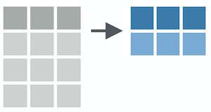
select()
Select columns with select()
select()
select(.data, ...)
.data = a data frame or tibble
. . . = One or more unquoted expressions separated by commas.
Variable names can be used as if they were positions in the data frame, so expressions like x:y can be used to select a range of variables.
penguins %>% filter(species == "Gentoo" & bill_length_mm > 55) %>% arrange(body_mass_g) %>% select(species:bill_depth_mm)## # A tibble: 3 x 4## species island bill_length_mm bill_depth_mm## <fct> <fct> <dbl> <dbl>## 1 Gentoo Biscoe 55.9 17## 2 Gentoo Biscoe 55.1 16## 3 Gentoo Biscoe 59.6 17penguins %>% filter(species == "Gentoo" & bill_length_mm > 55) %>% arrange(body_mass_g) %>% select(species, starts_with("bill_"))## # A tibble: 3 x 3## species bill_length_mm bill_depth_mm## <fct> <dbl> <dbl>## 1 Gentoo 55.9 17## 2 Gentoo 55.1 16## 3 Gentoo 59.6 17penguins %>% filter(species == "Gentoo" & bill_length_mm > 55) %>% arrange(body_mass_g) %>% select(ends_with("_mm"))## # A tibble: 3 x 3## bill_length_mm bill_depth_mm flipper_length_mm## <dbl> <dbl> <int>## 1 55.9 17 228## 2 55.1 16 230## 3 59.6 17 230Selection helpers
Selection helpers work in concert with select() to make it easier to select specific groups of variables.
Selection helpers
Selection helpers work in concert with select() to make it easier to select specific groups of variables.
Here are some commonly useful ones
everything(): Matches all variables.
last_col(): Select last variable, possibly with an offset.
starts_with(): Starts with a prefix.
ends_with(): Ends with a suffix.
contains(): Contains a literal string.
🔗 https://dplyr.tidyverse.org/reference/dplyr_tidy_select.html#overview-of-selection-features
mutate()
Create (or overwrite) variables with mutate()

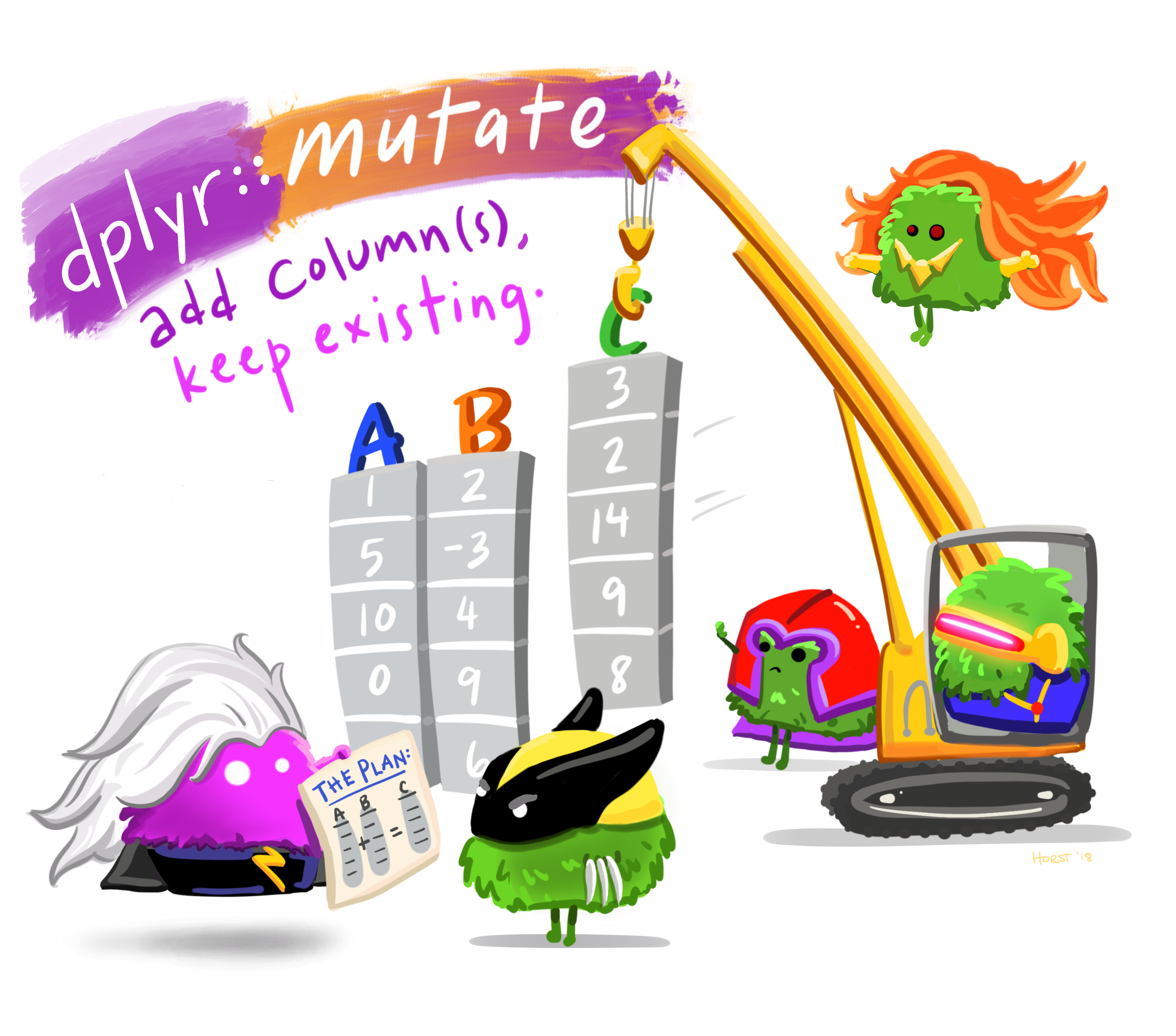
mutate()
mutate(.data, ...)
.data = a data frame or tibble
. . . = Name-value pairs. The name gives the name of the column in the output.
penguins %>% filter(species == "Gentoo" & bill_length_mm > 55) %>% arrange(body_mass_g) %>% select(starts_with("bill_")) %>% mutate(bill_length_m = bill_length_mm/1000)## # A tibble: 3 x 3## bill_length_mm bill_depth_mm bill_length_m## <dbl> <dbl> <dbl>## 1 55.9 17 0.0559## 2 55.1 16 0.0551## 3 59.6 17 0.0596penguins %>% filter(species == "Gentoo" & bill_length_mm > 55) %>% arrange(body_mass_g) %>% select(starts_with("bill_")) %>% mutate(bill_length_mm = as.character(bill_length_mm))## # A tibble: 3 x 2## bill_length_mm bill_depth_mm## <chr> <dbl>## 1 55.9 17## 2 55.1 16## 3 59.6 17
Your turn 2
04:00
In
ps_data, select only the variablesageandcondition.As we did with indexing in base R, you can use the minus sign (
-) to "de-select" columns. Keep everything inps_dataexceptsubidandcondition.Select the columns
correctandconditionwithout naming them, using their positions or de-selecting other variables.Use
mutate()to convertconditionfrom type "character" to type "factor". Then check that you've done this successfully. Hint: what function could you pipe to directly to check this?
Solution
ps_data %>% select(age, condition)## # A tibble: 588 x 2## age condition## <dbl> <chr> ## 1 2 Label ## 2 2 Label ## 3 2 Label ## 4 2 Label ## 5 2.13 Label ## 6 2.13 Label ## 7 2.13 Label ## 8 2.13 Label ## 9 2.32 Label ## 10 2.32 Label ## # … with 578 more rowsps_data %>% select(-c(subid, condition))## # A tibble: 588 x 3## item correct age## <chr> <int> <dbl>## 1 faces 1 2 ## 2 houses 1 2 ## 3 pasta 0 2 ## 4 beds 0 2 ## 5 beds 0 2.13## 6 faces 0 2.13## 7 houses 1 2.13## 8 pasta 1 2.13## 9 pasta 0 2.32## 10 faces 0 2.32## # … with 578 more rowsps_data %>% select(starts_with("c"))## # A tibble: 588 x 2## correct condition## <int> <chr> ## 1 1 Label ## 2 1 Label ## 3 0 Label ## 4 0 Label ## 5 0 Label ## 6 0 Label ## 7 1 Label ## 8 1 Label ## 9 0 Label ## 10 0 Label ## # … with 578 more rowsps_data %>% mutate(condition = as.factor(condition)) %>% glimpse()## Rows: 588## Columns: 5## $ subid <chr> "M22", "M22", "M22", "M22", "T22", "T22", "T22", "T22", "T17", "T17", "T17", "T17", …## $ item <chr> "faces", "houses", "pasta", "beds", "beds", "faces", "houses", "pasta", "pasta", "fa…## $ correct <int> 1, 1, 0, 0, 0, 0, 1, 1, 0, 0, 0, 0, 0, 1, 1, 1, 0, 0, 1, 1, 1, 1, 0, 1, 1, 1, 1, 0, …## $ age <dbl> 2.00, 2.00, 2.00, 2.00, 2.13, 2.13, 2.13, 2.13, 2.32, 2.32, 2.32, 2.32, 2.38, 2.38, …## $ condition <fct> Label, Label, Label, Label, Label, Label, Label, Label, Label, Label, Label, Label, …Summarizing data
summarize()
summarize() reduces your raw data frame into to a smaller summary data frame that only contains the variables resulting from the summary functions that you specify within summarize()
summarize()
summarize() reduces your raw data frame into to a smaller summary data frame that only contains the variables resulting from the summary functions that you specify within summarize()
Summary functions take vectors as inputs and return single values as outputs

Common examples are mean(), sd(), max(), min(), sum(), etc...
summarize()
summarize(.data, ...)
.data = a data frame or tibble
. . . = Name-value pairs of summary functions. The name will be the name of the variable in the result.
penguins %>% summarize(mean_bill_length = mean(bill_length_mm, na.rm = TRUE), max_flipper_length = max(flipper_length_mm, na.rm = TRUE))## # A tibble: 1 x 2## mean_bill_length max_flipper_length## <dbl> <int>## 1 43.9 231group_by()
group_by() creates groups based on one or more variables in the data, and this affects any downstream operations -- most commonly, summarize()
group_by()
What happens if we combine group_by() and summarize()?
summarize()
Let's see a couple examples of how we can combine group_by() and summarize()
penguins %>% group_by(species) %>% summarize(mean_bill_length = mean(bill_length_mm, na.rm = TRUE))## `summarise()` ungrouping output (override with `.groups` argument)## # A tibble: 3 x 2## species mean_bill_length## <fct> <dbl>## 1 Adelie 38.8## 2 Chinstrap 48.8## 3 Gentoo 47.5penguins %>% group_by(species, island) %>% summarize(mean_bill_length = mean(bill_length_mm, na.rm = TRUE))## `summarise()` regrouping output by 'species' (override with `.groups` argument)## # A tibble: 5 x 3## # Groups: species [3]## species island mean_bill_length## <fct> <fct> <dbl>## 1 Adelie Biscoe 39.0## 2 Adelie Dream 38.5## 3 Adelie Torgersen 39.0## 4 Chinstrap Dream 48.8## 5 Gentoo Biscoe 47.5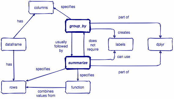
Your turn 3
07:00
From
ps_data, get the total number of correct trials for each subject and call this variablenum_correct. Hint: you can use the summary functionsum().Now get the total number of correct trials (
num_trials) for each unique combination ofconditionanditemand arrange the resulting rows by descending order ofnum_correct. Which combination of condition and item had the most/least correct responses?Lastly, calculate the proportion of correct responses for each
conditionand call this variableprop_correct(hint: becausecorrectis coded as 0 and 1, you can do this by taking the mean ofcorrect). In the same pipeline, create a bar plot that shows the differences between the mean proportion of correct responses between the two conditions, and color the bars by condition. What do you notice? (hint: it might be more straightforward to usegeom_colthangeom_bar)
Solution
# Q1. ps_data %>% group_by(subid) %>% summarize(num_correct = sum(correct))## `summarise()` ungrouping output (override with `.groups` argument)## # A tibble: 147 x 2## subid num_correct## <chr> <int>## 1 C1 4## 2 C10 2## 3 C11 3## 4 C12 3## 5 C13 2## 6 C14 3## 7 C15 4## 8 C16 2## 9 C17 2## 10 C18 3## # … with 137 more rows# Q2. ps_data %>% group_by(condition, item) %>% summarize(num_correct = sum(correct)) %>% arrange(desc(num_correct))## `summarise()` regrouping output by 'condition' (override with `.groups` argument)## # A tibble: 8 x 3## # Groups: condition [2]## condition item num_correct## <chr> <chr> <int>## 1 Label beds 60## 2 Label pasta 55## 3 Label faces 49## 4 Label houses 41## 5 No Label pasta 18## 6 No Label beds 15## 7 No Label faces 13## 8 No Label houses 12Q3. ps_data %>% group_by(condition) %>% summarize(prop_correct = mean(correct)) %>% ggplot(aes(x = prop_correct, y = condition, fill = condition)) + geom_col() + coord_flip()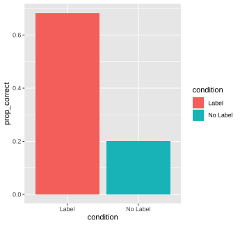
Column-wise operations
What if we want to apply dplyr verbs across multiple columns simultaneously? Check out these slides for more 👇
🔗 columnwise-operations-dplyr.netlify.app
Q & A
05:00
Next up...
Data tidying with tidyr
Break!
10:00