Step 1
.csv, .txt, .sav, etc.)You need to call a function that works with a particular data format (.csv, .txt, .sav, etc.)
You need to tell R where to look for the data
readr
read_csv(), read_tsv(), read_delim(), read_fwf(), etc...
readr
read_csv(), read_tsv(), read_delim(), read_fwf(), etc...
rio
import()
readr
read_csv(), read_tsv(), read_delim(), read_fwf(), etc...
rio
import()
✅
rio::import()We just call import() and under the hood it calls the right read function given the file's extension (.csv, .txt, .sav, .xlsx, etc.)
rio::import()We just call import() and under the hood it calls the right read function given the file's extension (.csv, .txt, .sav, .xlsx, etc.)
We'll get some practice with this in a few minutes
When R looks for a file, it has a starting point. This is called the working directory.
When R looks for a file, it has a starting point. This is called the working directory.
The working directory that you're currently in is displayed in the console window and the files tab. Let's take a look in RStudio...
When R looks for a file, it has a starting point. This is called the working directory.
The working directory that you're currently in is displayed in the console window and the files tab. Let's take a look in RStudio...
If you ever get lost, you can print your working directory with getwd()
When R looks for a file, it has a starting point. This is called the working directory.
The working directory that you're currently in is displayed in the console window and the files tab. Let's take a look in RStudio...
If you ever get lost, you can print your working directory with getwd()
If you are working in a .Rmd document, R by default will set whatever folder on your computer where that .Rmd file lives as your working directory
getwd()## [1] "/Users/bcullen/Desktop/summeR-bootcamp-2020/static/slides"For example, I created these slides in a .Rmd document that lives in this folder on my computer ☝️
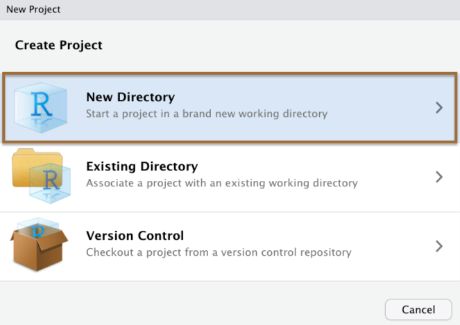
The best way to simplify issues with working directories is to use RStudio Projects.
The best way to simplify issues with working directories is to use RStudio Projects.
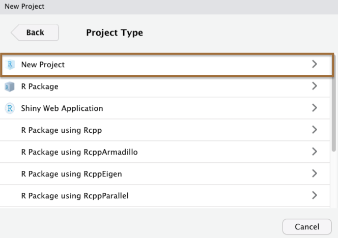
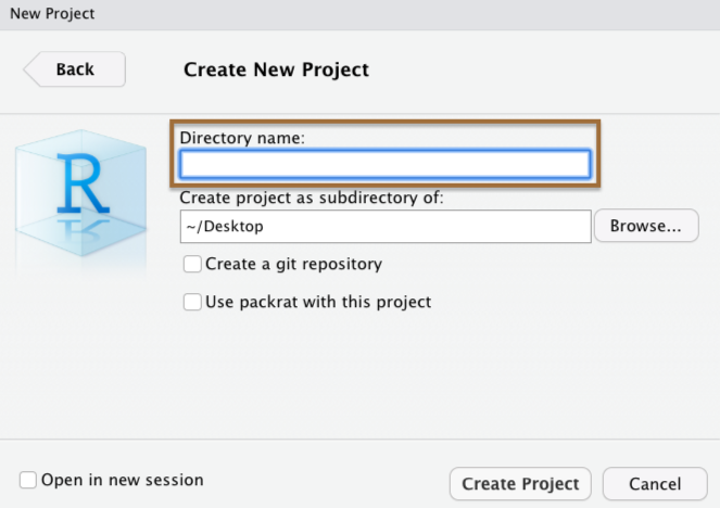
When you create a Project in RStudio, it is associated with a folder somewhere on your computer.
When you create a Project in RStudio, it is associated with a folder somewhere on your computer.
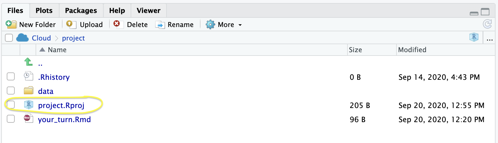
It will automatically create a .Rproj file in that folder, which will keep track of the "top level" of your project.
When you create a Project in RStudio, it is associated with a folder somewhere on your computer.
It will automatically create a .Rproj file in that folder, which will keep track of the "top level" of your project.
For example, we've been using RStudio Projects for "Your Turn" exercises
here::here()here::here()In combination with RStudio Projects, use the here package
here::here() will build a file path to the top level of your project directory.
This makes it easy to tell R where files live relative to the top-level folder of your project

04:00
rio and here packages.pragmatic_scales_data.csv. Why do you get an error? Where is this file saved? Hint: Look through the folder(s) in the Files paneps_data <- import("pragmatic_scales_data.csv")here() functionrio is flexible with file types -- rio::import() will call the right function under the hood to read in the file based on the file extension. Use rio to import pragmatic_scales_data.sav (an SPSS file type) and save it to a new object named ps_data_2.# Q1.library(rio)library(here)# Q2. ps_data <- import("pragmatic_scales_data.csv")## Error in import("pragmatic_scales_data.csv"): No such fileThe file pragmatic_scales_data.csv is saved in the data folder, so we need to tell R to look in that folder.
# Q3.ps_data <- import(here("data/pragmatic_scales_data.csv"))# Q4.ps_data_2 <- import(here("data/pragmatic_scales_data.sav"))You can also use rio to export your data using export(), saving it in any of the formats that it works with.
You can also use rio to export your data using export(), saving it in any of the formats that it works with.
Here are the arguments you will need to use for export()
export(x, file)You can also use rio to export your data using export(), saving it in any of the formats that it works with.
Here are the arguments you will need to use for export()
export(x, file)x is the data.frame object in your RStudio Environment you want to export
You can also use rio to export your data using export(), saving it in any of the formats that it works with.
Here are the arguments you will need to use for export()
export(x, file)x is the data.frame object in your RStudio Environment you want to export
file is the path/filename for the resulting file
For example, let's say I want to export ps_data as an .xlsx file and put it into the data/ subdirectory.
export(ps_data, here::here("data/ps_data.xlsx"))04:00
Look through the Files pane and find the file another_data_set.csv. Make note of what subdirectory it is saved in. Import the data and save to an object called another_df.
Now export the data you just imported and save it into the data/ directory. Make sure the name of the resulting file is another_data_set, and export it as a .xlsx file.
One of your colleagues insists you send them a .sav file so that they can run the analyses in SPSS. Make another copy of another_data_set in the data/ subdirectory that is in the .sav format.
Finally, let's read one of these datasets to make sure everything worked as expected. Import another_data_set.sav , which you just created, and import it, saving it to a new object named another_df_2.
Now that your data is loaded in R, you'll want to take a look at it. There are a few different ways to do that, which each offer different information.
Now that your data is loaded in R, you'll want to take a look at it. There are a few different ways to do that, which each offer different information.
View()One way is to click on the View button in the environment pane...
Now that your data is loaded in R, you'll want to take a look at it. There are a few different ways to do that, which each offer different information.
View()One way is to click on the View button in the environment pane...
You should see ps_data in the environment pane with a little data table icon at the far right. Click on that icon.
You'll notice that this ran View(ps_data) in the console. We could have instead just typed this directly ourselves -- notice the capital V in View() 👀
head() and tail()head() and tail()You can also see just the first few rows of a dataframe with head(), which is especially helpful for large data sets
head(ps_data)## subid item correct age condition## 1 M22 faces 1 2.00 Label## 2 M22 houses 1 2.00 Label## 3 M22 pasta 0 2.00 Label## 4 M22 beds 0 2.00 Label## 5 T22 beds 0 2.13 Label## 6 T22 faces 0 2.13 Labeltail() is the complement to head(), displaying just the final rows from a dataframe
tail(ps_data)## subid item correct age condition## 583 MSCH84 pasta 1 2.83 No Label## 584 MSCH84 beds 0 2.83 No Label## 585 MSCH85 faces 0 2.69 No Label## 586 MSCH85 houses 0 2.69 No Label## 587 MSCH85 pasta 0 2.69 No Label## 588 MSCH85 beds 0 2.69 No Labelstr() and glimpse()We saw str() when we first introduced data frames. It's worth mentioning it again because it can be so useful when you import data to see how your variables were read in (i.e. their types)
str(ps_data)## 'data.frame': 588 obs. of 5 variables:## $ subid : chr "M22" "M22" "M22" "M22" ...## $ item : chr "faces" "houses" "pasta" "beds" ...## $ correct : int 1 1 0 0 0 0 1 1 0 0 ...## $ age : num 2 2 2 2 2.13 2.13 2.13 2.13 2.32 2.32 ...## $ condition: chr "Label" "Label" "Label" "Label" ...glimpse() is very similar to str() but is a tidyverse function, and it shows you a little more raw data
glimpse(ps_data)## Rows: 588## Columns: 5## $ subid <chr> "M22", "M22", "M22", "M22", "T22", "T22", "T22", "T22", "T1…## $ item <chr> "faces", "houses", "pasta", "beds", "beds", "faces", "house…## $ correct <int> 1, 1, 0, 0, 0, 0, 1, 1, 0, 0, 0, 0, 0, 1, 1, 1, 0, 0, 1, 1,…## $ age <dbl> 2.00, 2.00, 2.00, 2.00, 2.13, 2.13, 2.13, 2.13, 2.32, 2.32,…## $ condition <chr> "Label", "Label", "Label", "Label", "Label", "Label", "Labe…02:00
Take a look at another_df, which should be saved in your Global Environment. Click the "View" button in the Environment pane, and also use View() in your Console.
Now look at some summary information about another_df using str() and glimpse(). Hint. You will need to load the tidyverse package first in order to use glimpse().
Lastly find the number of rows and columns in another_df using nrow() and ncol(), respectively. Make sure your answers match the summary information given to you above.
View(another_df)library(tidyverse)str(another_df)## 'data.frame': 32 obs. of 4 variables:## $ subid : chr "A001" "A001" "A001" "A001" ...## $ stimuli: chr "A" "B" "C" "D" ...## $ correct: int 0 0 1 0 1 1 1 1 0 0 ...## $ age : num 2.5 2.5 2.5 2.5 2.75 2.75 2.75 2.75 3.6 3.6 ...glimpse(another_df)## Rows: 32## Columns: 4## $ subid <chr> "A001", "A001", "A001", "A001", "B002", "B002", "B002", "B002…## $ stimuli <chr> "A", "B", "C", "D", "A", "B", "C", "D", "A", "B", "C", "D", "…## $ correct <int> 0, 0, 1, 0, 1, 1, 1, 1, 0, 0, 1, 1, 1, 1, 1, 1, 0, 0, 0, 0, 1…## $ age <dbl> 2.50, 2.50, 2.50, 2.50, 2.75, 2.75, 2.75, 2.75, 3.60, 3.60, 3…nrow(another_df)## [1] 32ncol(another_df)## [1] 405:00
ggplot210:00
Keyboard shortcuts
| ↑, ←, Pg Up, k | Go to previous slide |
| ↓, →, Pg Dn, Space, j | Go to next slide |
| Home | Go to first slide |
| End | Go to last slide |
| Number + Return | Go to specific slide |
| b / m / f | Toggle blackout / mirrored / fullscreen mode |
| c | Clone slideshow |
| p | Toggle presenter mode |
| t | Restart the presentation timer |
| ?, h | Toggle this help |
| o | Tile View: Overview of Slides |
| Esc | Back to slideshow |
.csv, .txt, .sav, etc.)You need to call a function that works with a particular data format (.csv, .txt, .sav, etc.)
You need to tell R where to look for the data
readr
read_csv(), read_tsv(), read_delim(), read_fwf(), etc...
readr
read_csv(), read_tsv(), read_delim(), read_fwf(), etc...
rio
import()
readr
read_csv(), read_tsv(), read_delim(), read_fwf(), etc...
rio
import()
✅
rio::import()We just call import() and under the hood it calls the right read function given the file's extension (.csv, .txt, .sav, .xlsx, etc.)
rio::import()We just call import() and under the hood it calls the right read function given the file's extension (.csv, .txt, .sav, .xlsx, etc.)
We'll get some practice with this in a few minutes
When R looks for a file, it has a starting point. This is called the working directory.
When R looks for a file, it has a starting point. This is called the working directory.
The working directory that you're currently in is displayed in the console window and the files tab. Let's take a look in RStudio...
When R looks for a file, it has a starting point. This is called the working directory.
The working directory that you're currently in is displayed in the console window and the files tab. Let's take a look in RStudio...
If you ever get lost, you can print your working directory with getwd()
When R looks for a file, it has a starting point. This is called the working directory.
The working directory that you're currently in is displayed in the console window and the files tab. Let's take a look in RStudio...
If you ever get lost, you can print your working directory with getwd()
If you are working in a .Rmd document, R by default will set whatever folder on your computer where that .Rmd file lives as your working directory
When R looks for a file, it has a starting point. This is called the working directory.
The working directory that you're currently in is displayed in the console window and the files tab. Let's take a look in RStudio...
If you ever get lost, you can print your working directory with getwd()
If you are working in a .Rmd document, R by default will set whatever folder on your computer where that .Rmd file lives as your working directory
getwd()## [1] "/Users/bcullen/Desktop/summeR-bootcamp-2020/static/slides"For example, I created these slides in a .Rmd document that lives in this folder on my computer ☝️
The best way to simplify issues with working directories is to use RStudio Projects.
The best way to simplify issues with working directories is to use RStudio Projects.
When you create a Project in RStudio, it is associated with a folder somewhere on your computer.
When you create a Project in RStudio, it is associated with a folder somewhere on your computer.
It will automatically create a .Rproj file in that folder, which will keep track of the "top level" of your project.
When you create a Project in RStudio, it is associated with a folder somewhere on your computer.
It will automatically create a .Rproj file in that folder, which will keep track of the "top level" of your project.
For example, we've been using RStudio Projects for "Your Turn" exercises
here::here()here::here()In combination with RStudio Projects, use the here package
here::here() will build a file path to the top level of your project directory.
This makes it easy to tell R where files live relative to the top-level folder of your project
04:00
rio and here packages.pragmatic_scales_data.csv. Why do you get an error? Where is this file saved? Hint: Look through the folder(s) in the Files paneps_data <- import("pragmatic_scales_data.csv")here() functionrio is flexible with file types -- rio::import() will call the right function under the hood to read in the file based on the file extension. Use rio to import pragmatic_scales_data.sav (an SPSS file type) and save it to a new object named ps_data_2.# Q1.library(rio)library(here)# Q2. ps_data <- import("pragmatic_scales_data.csv")## Error in import("pragmatic_scales_data.csv"): No such fileThe file pragmatic_scales_data.csv is saved in the data folder, so we need to tell R to look in that folder.
# Q3.ps_data <- import(here("data/pragmatic_scales_data.csv"))# Q4.ps_data_2 <- import(here("data/pragmatic_scales_data.sav"))You can also use rio to export your data using export(), saving it in any of the formats that it works with.
You can also use rio to export your data using export(), saving it in any of the formats that it works with.
Here are the arguments you will need to use for export()
export(x, file)You can also use rio to export your data using export(), saving it in any of the formats that it works with.
Here are the arguments you will need to use for export()
export(x, file)x is the data.frame object in your RStudio Environment you want to export
You can also use rio to export your data using export(), saving it in any of the formats that it works with.
Here are the arguments you will need to use for export()
export(x, file)x is the data.frame object in your RStudio Environment you want to export
file is the path/filename for the resulting file
You can also use rio to export your data using export(), saving it in any of the formats that it works with.
Here are the arguments you will need to use for export()
export(x, file)x is the data.frame object in your RStudio Environment you want to export
file is the path/filename for the resulting file
For example, let's say I want to export ps_data as an .xlsx file and put it into the data/ subdirectory.
export(ps_data, here::here("data/ps_data.xlsx"))04:00
Look through the Files pane and find the file another_data_set.csv. Make note of what subdirectory it is saved in. Import the data and save to an object called another_df.
Now export the data you just imported and save it into the data/ directory. Make sure the name of the resulting file is another_data_set, and export it as a .xlsx file.
One of your colleagues insists you send them a .sav file so that they can run the analyses in SPSS. Make another copy of another_data_set in the data/ subdirectory that is in the .sav format.
Finally, let's read one of these datasets to make sure everything worked as expected. Import another_data_set.sav , which you just created, and import it, saving it to a new object named another_df_2.
Now that your data is loaded in R, you'll want to take a look at it. There are a few different ways to do that, which each offer different information.
Now that your data is loaded in R, you'll want to take a look at it. There are a few different ways to do that, which each offer different information.
View()One way is to click on the View button in the environment pane...
Now that your data is loaded in R, you'll want to take a look at it. There are a few different ways to do that, which each offer different information.
View()One way is to click on the View button in the environment pane...
You should see ps_data in the environment pane with a little data table icon at the far right. Click on that icon.
Now that your data is loaded in R, you'll want to take a look at it. There are a few different ways to do that, which each offer different information.
View()One way is to click on the View button in the environment pane...
You should see ps_data in the environment pane with a little data table icon at the far right. Click on that icon.
You'll notice that this ran View(ps_data) in the console. We could have instead just typed this directly ourselves -- notice the capital V in View() 👀
head() and tail()head() and tail()You can also see just the first few rows of a dataframe with head(), which is especially helpful for large data sets
head(ps_data)## subid item correct age condition## 1 M22 faces 1 2.00 Label## 2 M22 houses 1 2.00 Label## 3 M22 pasta 0 2.00 Label## 4 M22 beds 0 2.00 Label## 5 T22 beds 0 2.13 Label## 6 T22 faces 0 2.13 Labeltail() is the complement to head(), displaying just the final rows from a dataframe
tail(ps_data)## subid item correct age condition## 583 MSCH84 pasta 1 2.83 No Label## 584 MSCH84 beds 0 2.83 No Label## 585 MSCH85 faces 0 2.69 No Label## 586 MSCH85 houses 0 2.69 No Label## 587 MSCH85 pasta 0 2.69 No Label## 588 MSCH85 beds 0 2.69 No Labelstr() and glimpse()We saw str() when we first introduced data frames. It's worth mentioning it again because it can be so useful when you import data to see how your variables were read in (i.e. their types)
str(ps_data)## 'data.frame': 588 obs. of 5 variables:## $ subid : chr "M22" "M22" "M22" "M22" ...## $ item : chr "faces" "houses" "pasta" "beds" ...## $ correct : int 1 1 0 0 0 0 1 1 0 0 ...## $ age : num 2 2 2 2 2.13 2.13 2.13 2.13 2.32 2.32 ...## $ condition: chr "Label" "Label" "Label" "Label" ...glimpse() is very similar to str() but is a tidyverse function, and it shows you a little more raw data
glimpse(ps_data)## Rows: 588## Columns: 5## $ subid <chr> "M22", "M22", "M22", "M22", "T22", "T22", "T22", "T22", "T1…## $ item <chr> "faces", "houses", "pasta", "beds", "beds", "faces", "house…## $ correct <int> 1, 1, 0, 0, 0, 0, 1, 1, 0, 0, 0, 0, 0, 1, 1, 1, 0, 0, 1, 1,…## $ age <dbl> 2.00, 2.00, 2.00, 2.00, 2.13, 2.13, 2.13, 2.13, 2.32, 2.32,…## $ condition <chr> "Label", "Label", "Label", "Label", "Label", "Label", "Labe…02:00
Take a look at another_df, which should be saved in your Global Environment. Click the "View" button in the Environment pane, and also use View() in your Console.
Now look at some summary information about another_df using str() and glimpse(). Hint. You will need to load the tidyverse package first in order to use glimpse().
Lastly find the number of rows and columns in another_df using nrow() and ncol(), respectively. Make sure your answers match the summary information given to you above.
View(another_df)library(tidyverse)str(another_df)## 'data.frame': 32 obs. of 4 variables:## $ subid : chr "A001" "A001" "A001" "A001" ...## $ stimuli: chr "A" "B" "C" "D" ...## $ correct: int 0 0 1 0 1 1 1 1 0 0 ...## $ age : num 2.5 2.5 2.5 2.5 2.75 2.75 2.75 2.75 3.6 3.6 ...glimpse(another_df)## Rows: 32## Columns: 4## $ subid <chr> "A001", "A001", "A001", "A001", "B002", "B002", "B002", "B002…## $ stimuli <chr> "A", "B", "C", "D", "A", "B", "C", "D", "A", "B", "C", "D", "…## $ correct <int> 0, 0, 1, 0, 1, 1, 1, 1, 0, 0, 1, 1, 1, 1, 1, 1, 0, 0, 0, 0, 1…## $ age <dbl> 2.50, 2.50, 2.50, 2.50, 2.75, 2.75, 2.75, 2.75, 3.60, 3.60, 3…nrow(another_df)## [1] 32ncol(another_df)## [1] 405:00
ggplot210:00